The S&P 500 is not a market I include in my diversified commodity futures portfolio. Why? – Because it doesn’t move like other commodities or futures.
Trends are constantly backtracked causing many smaller swings within the larger trend. It’s a mean reversion market that spends much of it’s time oscillating up and down, crossing through an equilibrium level.
Strong directional moves are more likely to be followed by a counter reaction rather than an immediate continuation of that move. So trying to chase new trends just does not work well when trading stock market indexes.
With these characteristics in mind, the first step to creating a tradable system for the e-mini s&P 500 is to define an equilibrium point and then measure the distribution of price around that level.
Mapping Price Distribution
Using a very short moving average of median price does a good job of defining a usable equilibrium point. A distribution can then be calculated around that equilibrium by subtracting the equilibrium point from the market price.
To normalize these readings for volatility, this result is then divided by the recent daily range of price. The result looks like this…
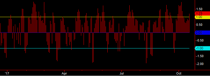
MA Distribution
The +1 and -1 lines are drawn on the chart to provide a reference to scale. Notice how moves beyond these lines quickly retrace to pass through the equilibrium at the zero line. Often this retreat swings all the way to the other end of the spectrum in just a few days.
Trend Direction
The MA Distribution tells us what’s happening in the very short term using just a couple weeks of data. A trend calculation tells us what’s happening with a much wider view. We need this trend measure to define the “Big Picture” while the MA Distribution tells us what’s happening now, in a tradeable timeframe.
A simple moving average of the last 6 to 9 months will be used to reference the trend. When closing price is above this moving average, the Trend is Up, and when the close is below the moving average, the Trend is Down.
When the trend is Up, the system will take long trades only
When the trend is Down, the system will take short trades only.
Trading the Pullbacks
When price is trending directionally, the odds are it will continue in that direction. What we don’t want to do is jump on the trend when it’s making new extremes. Instead, we will enter on pullbacks to the larger trend.
The Trend Direction will define the trade direction and the MA Distribution will provide the trigger to enter the market during significant pullbacks to the major trend.
Buy Signal = Trend Direction is Up and the MA Distribution registers a significant Pullback, i.e, negative value.
Sell Signal = Trend Direction is Down and the MA Distribution registers a significant Pullback, i.e, positive value.
Exiting the trade
The exit is where the money is made. Figuring out where to enter is the easy part, finding a good exit is always a challenge.
I like to start with same logic used on the entry when searching for a good exit. And for this system the Equilibrium point seems like a logical exit. The observation explained in the beginning about S&P price continuously crossing through the equilibrium point, moving from one extreme to the other, is what we want to capture.
Enter at the extremes and exit at equilibrium follows that initial observation.
Exit for Long and Short trades = MA Distribution crosses zero.
Price doesn’t always go from one extreme to the other but it does repeatedly go back and touch equilibrium.
Trade Performance
For the initial run I’ll just use single contracts. For each Buy and Sell signal the system will trade 1 contract. Only one Long entry or one Short entry will be allowed at a time. This means that If the system is Long and then another buy entry is triggered, it will be ignored since the system already has a long position. Same for the Short side.
Symbol – ES
Equity – $10,000
History – 10 years
Trading Costs – $20 per trade
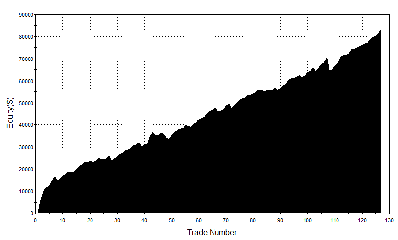
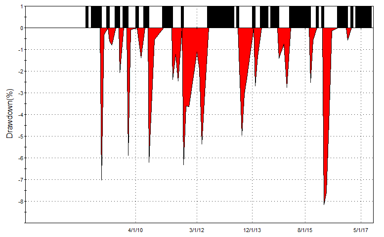
Both the equity curve and the percent drawdown look good. All drawdowns were contained within 8% of the previous equity high. But this is on a one contract basis so the drawdown percent doesn’t mean too much since we are not compounding the profits.
Position Sizing
Obviously we would not trade one contract per trade for 10 years straight. Instead, the number of contracts to trade for each signal should be calculated based on account equity and/or position risk. Over time, this will result in an increase of position size as equity increases.
And just as importantly, the position size will be decreased when equity is contracting, and/or, position risk increases. This position sizing serves to “normalize”all trades over time by scaling up and down contracts per trade in response to price volatility and/or available equity.
In this case we are dealing with just one symbol but we still want to normalize the price volatility on a trade by trade basis to make all trades as equal as possible, regardless of current price volatility.
This can be accomplished by calculating a dollar risk using the recent average daily price range multiplied by the E-mini S&P dollar point value. Next we determine the percentage of equity to risk per trade and divide that by the dollar risk. From there we can calculate the position size for each trade.
The performance results based on 5% risk per trade and 10% risk per trade are as follows…
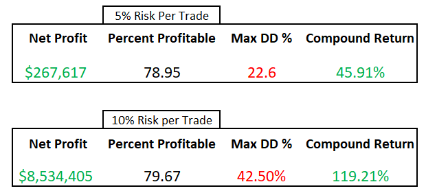
At 5% the max drawdown is 22.6%. For some that might not be enough risk so in the second run I increased it to 10%. Now the max drawdown is 42% which might be too much for some. I’m sure most of you can find a balance somewhere on that spectrum.
Either way, the range of Compounded Average Growth Rates between 45.91 and 119.21 are fantastic. Especially considering this is a single market system that doesn’t benefit from portfolio diversification.
These results were derived using a starting equity of $10,000. Starting with more would be ideal because at 10k you may not be able to take all the trades in the beginning.
But here’s a better idea, even if you have sufficient starting capital, use options to reduce risk and increase return on investment. The S&P 500 offers excellent option spread opportunities because of the constant steep volatility skew.
Combine that with trade signals that are almost 80% accurate and the returns could be even better than trading the futures contracts. The average hold time for this system is 6 days so debit spreads are perfectly suitable to trade.
TradeStation code and Spreadsheet calculator
If you are interested in trading this system I’ve put together a download with everything you need. No special software is needed, just price data for the S&P 500. Plug a few values into the provided spreadsheet and the trade entries and exits are calculated for you.
The TradeStation ELD is provided if you want to do more testing. The EasyLanguage code is also saved in a text file which can be used to load into MultiCharts software or used as pseudo code if you want to code this system for another platform.
The money management algorithm used to calculate the compounded results is a part of the easylanguage file. It can be turned on or off as an input on the strategy settings.
Buy Now – $45
This is an instant digital download. After payment check your paypal email for download instructions. Check your spam/junk folders if you don’t see the email right away.
Good trading,
Shay